B.14 Text with geom_text

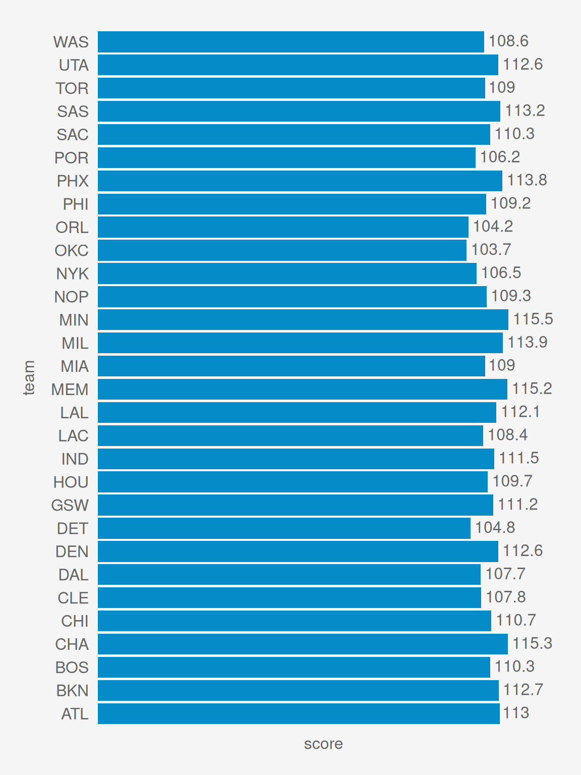
We can add text to a plot using label aesthetic and geom_text. Let’s add text to the bar plot we made after aggregating the data.

Code

dg = dd %>% 
  group_by(team) %>%
  summarise(score = round(mean(score),1)) 

g = ggplot(dg, aes(x = score, 
                   y = team, 
                   label = score))+
  geom_col(color = NA)+
  geom_text(hjust = -0.1, 
            vjust =  0.4)

g %>% 
  pub(type = 'bar')

[1] 85.89991
[1] 80
[1] 20
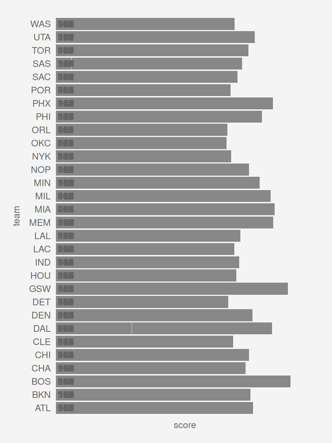
[1] 185.8999

Note that without aggregating the bar plot looks the same, but it will plot separate text for each row in the data, and all the text will be overlapping along the left.

Code

g = ggplot(dd, aes(x = score, 
                   y = team, 
                   label = score))+
  geom_col(color = NA, 
           fill  = pubmediumgray)+
  geom_text(hjust = 0)

g %>% 
  pub(type = 'bar')

[1] 85.89991
[1] 80
[1] 20
[1] 185.8999

To use geom_text with position_dodge, add label like before, but also add group.

Code

dg = dd %>%
  group_by(team, season.type) %>%
  summarise(score = sum(score), 
            .groups = 'keep')

post.teams = unique(dg$team[dg$season.type == 'post'])
dg = dg %>% filter(team %in% post.teams)

g = ggplot(dg, aes(x = score, 
                   y = team, 
                   fill  = season.type, 
                   label = score, 
                   group = season.type))+
  geom_col(position = position_dodge(width = .9), 
           color = NA)+
  geom_text(hjust = -.1, 
            vjust = 0.3, 
            position = position_dodge(width = .9))

g %>% 
  pub(type = 'bar')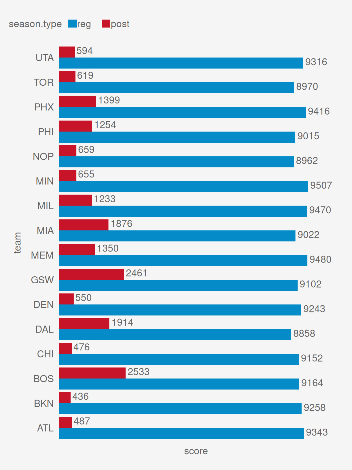

[1] 85.89991
[1] 80
[1] 20
[1] 185.8999

You can use geom_text with geom_point, geom_line, etc as well.