13.9 Errors in variables, total least squares

When predictors \(x_1, x_2, \ldots, x_p\) are estimates and have errors, and are not known exactly the OLS estimates are biased. The total least squares method can be used to estimate the coefficients.

Suppose that \(y\) is linearly related to some \(x\) plus some error (like simple linear regression) but we only known \(x.star\), which is \(x\) with some noise.

Code

## Simulate data
set.seed(1)
n = 10000
x = rnorm(n)
y = .5 + 1*x + rnorm(n) ## true relationship
x.star = x + 2*rnorm(n) ## noisy x
df = data.frame(y, x, x.star)

## Visualize
dg = df %>%
  pivot_longer(cols = c(x, x.star))

g = ggplot(dg, 
       aes(x = value, 
           y = y, 
           color = name))+
  geom_point() +
  facet_wrap(~name)

g %>% 
  pub(xlim = c(-8, 8), 
      ylim = c(-8, 8))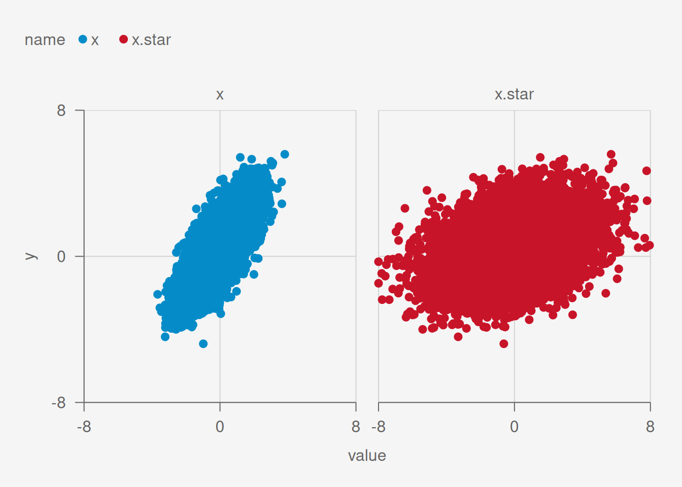

[1] 31.97542
[1] 80
[1] 20
[1] 131.9754

Now let’s show how the OLS estimates are different.

Code

## OLS
lm1 = lm(y ~ x     , data = df)
lm2 = lm(y ~ x.star, data = df)
summary(lm1)$coefficients
summary(lm2)$coefficients ## slope is underestimated

             Estimate  Std. Error   t value Pr(>|t|)
(Intercept) 0.4958409 0.009908363  50.04267        0
x           1.0047418 0.009787710 102.65341        0
             Estimate  Std. Error  t value      Pr(>|t|)
(Intercept) 0.4875360 0.013445164 36.26107 1.334407e-270
x.star      0.2026182 0.005963395 33.97699 1.440827e-239

The intercept is similar in both cases. Both are near 0.5. However the slope is much different in the second model with the noisy version of \(x\). In particular the slope is underestimated.

Code

summary(lm1)$r.squared
summary(lm2)$r.squared

[1] 0.5131411
[1] 0.1035142

Now let’s use total least squares.

Code

## Total least squares
tls = lm(y ~ x + x.star, data = df)