B.12 Color bars using fill

We can also use color our bars using the fill aesthetic.

Code

g = ggplot(dd, aes(x = score, 
                   y = team, 
                   fill = season.type))+
  geom_col(color = NA)

g %>% 
  pub(type = 'bar')

[1] 85.89991
[1] 80
[1] 20
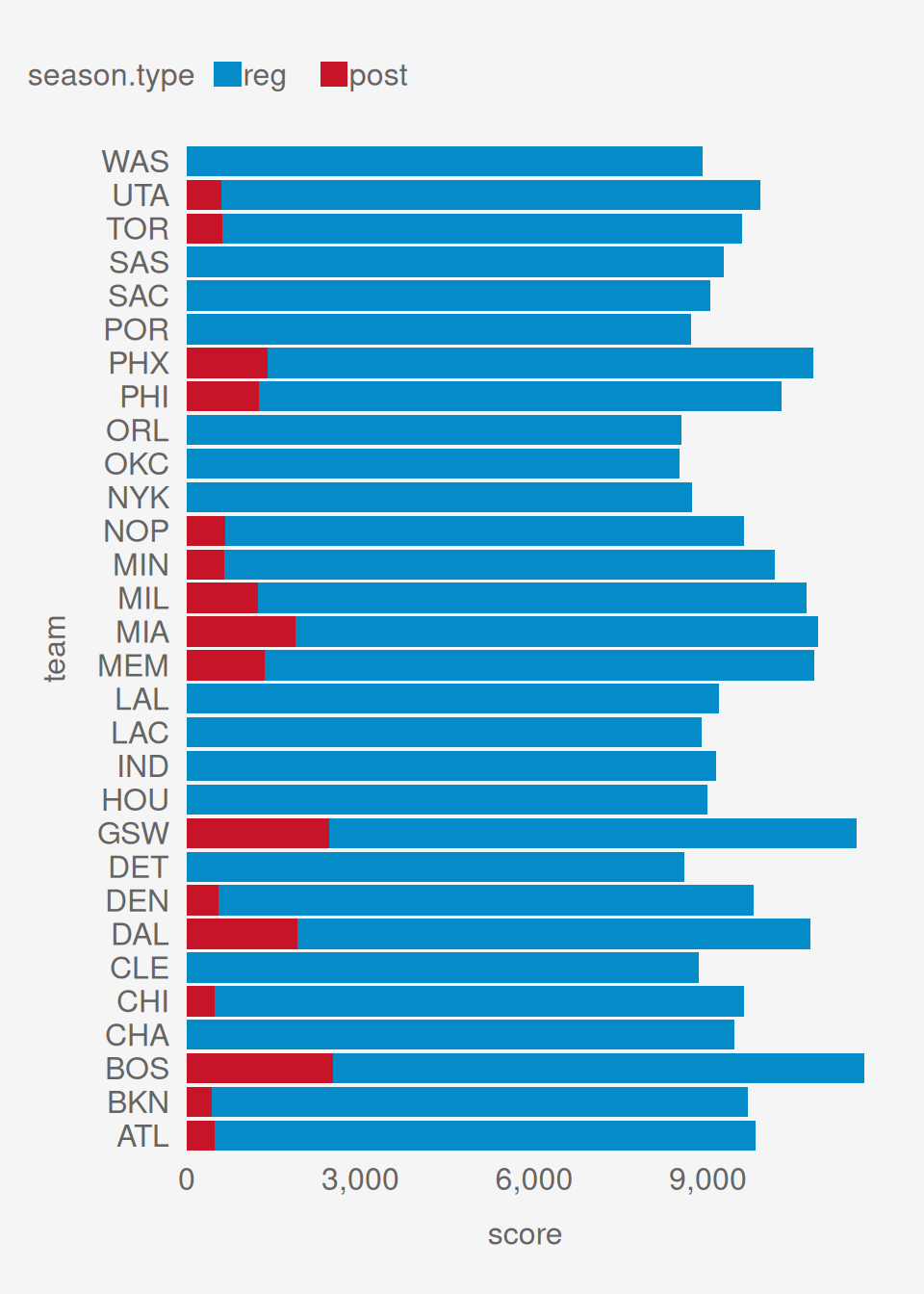
[1] 185.8999

Typically you use fill. Note that color affects only the border.

Code

g = ggplot(dd, aes(x = score, 
                   y = team, 
                   color = season.type))+
  geom_col()

g %>% 
  pub(type = 'bar')

[1] 85.89991
[1] 80
[1] 20
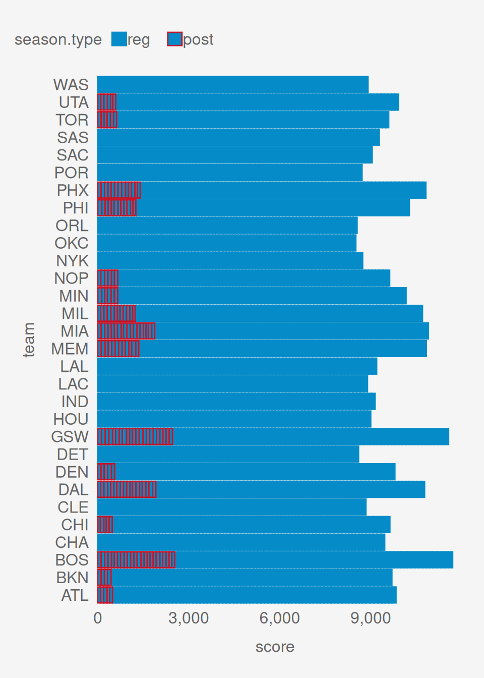
[1] 185.8999

That’s not ideal. It is drawing a little bar for each individual game and then stacking them together. In most cases we probably want to aggregate the data first like this:

Code

dg = dd %>%
  group_by(team, season.type) %>%
  summarise(score = sum(score), 
            .groups = 'keep')

g = ggplot(dg, aes(x = score, 
                   y = team, 
                   fill = season.type))+
  geom_col(color = NA)

g %>% 
  pub(type = 'bar')

[1] 85.89991
[1] 80
[1] 20
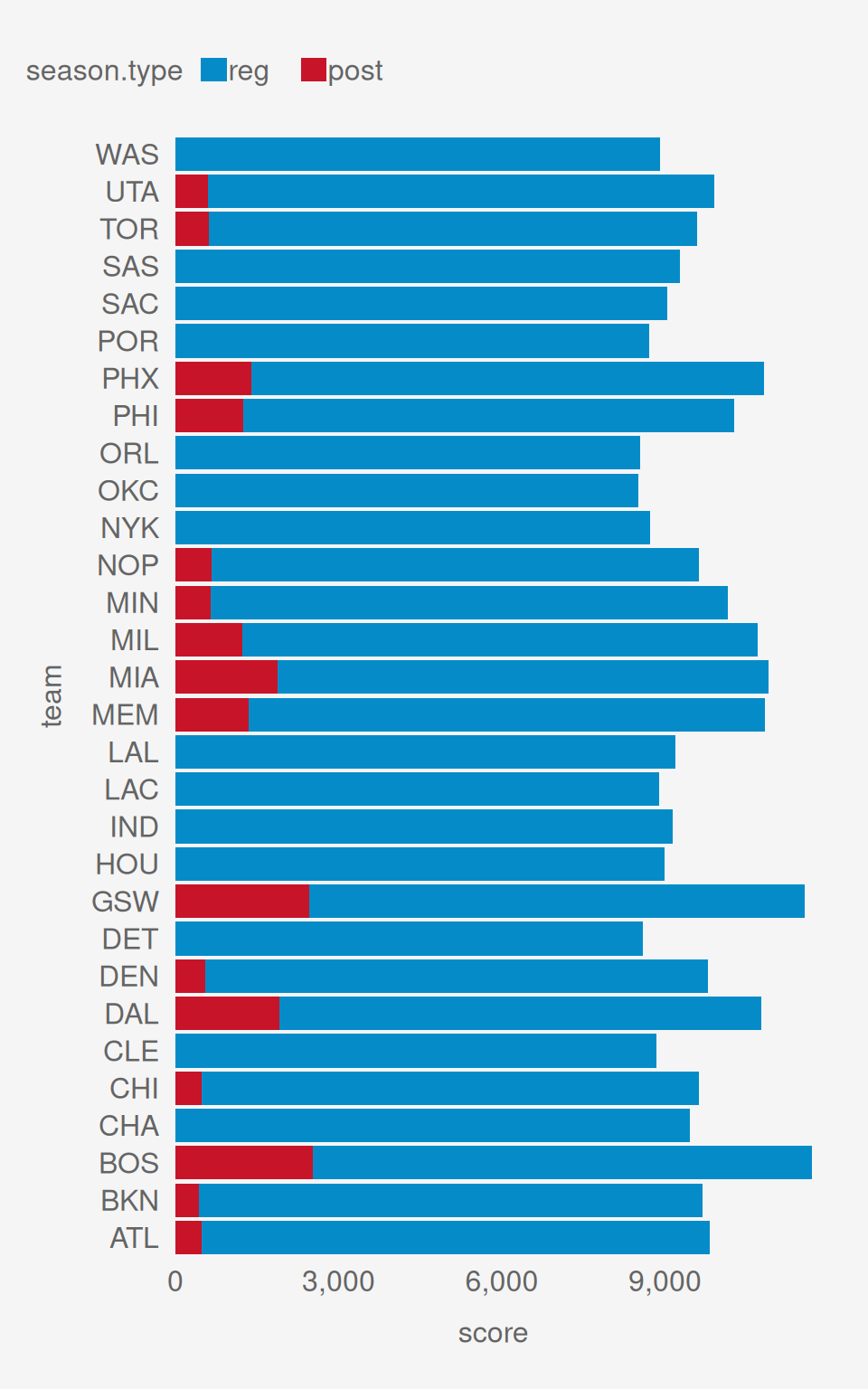
[1] 185.8999

You may often use fill and not notice this issue, but it is something to be aware of.

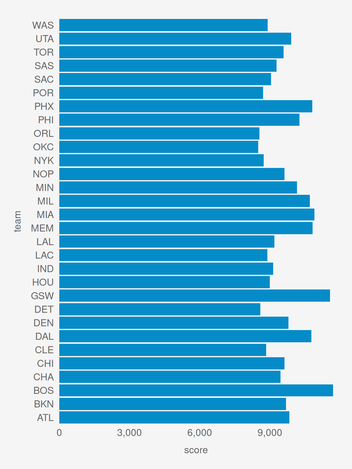
Even with our first bar plot it would be better to aggregate first for reasons we’ll see when we try to use geom_text below. This plot looks the same, but there is one bar per team instead of one bar per game:

Code

dg = dd %>% 
  group_by(team) %>%
  summarise(score = sum(score)) 

g = ggplot(dg, aes(x = score, 
                   y = team))+
  geom_col(color = NA)

g %>% 
  pub(type = 'bar')

[1] 85.89991
[1] 80
[1] 20
[1] 185.8999