4.6 Formatting with pubtheme

4.6 Formatting with `pubtheme`

The previous plot was functional and told us what we wanted to know. But let’s start using pubtheme. We’ll copy and paste the scatter plot code from https://github.com/bmacGTPM/pubtheme and edit it for our data.

Code

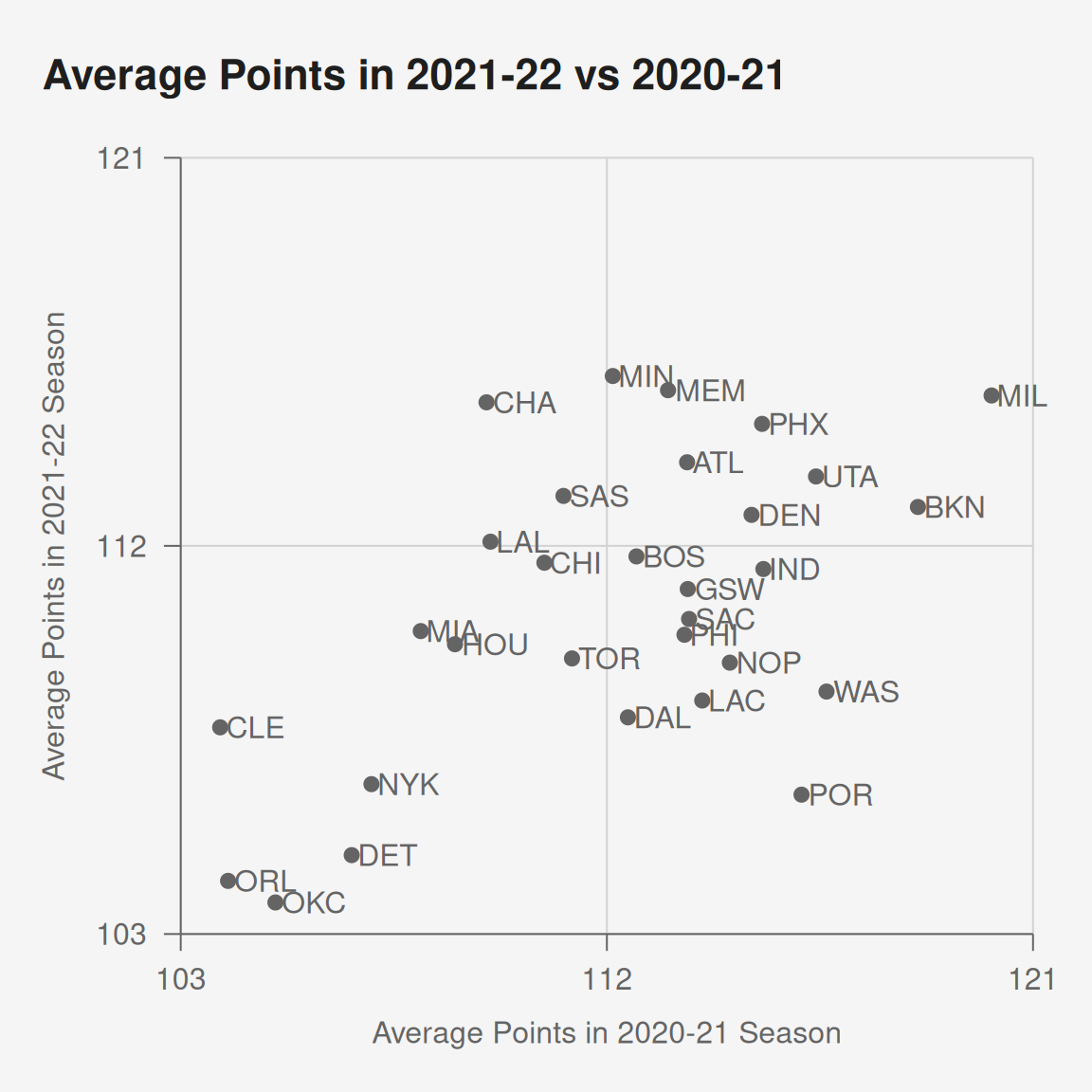
title = 'Average Points in 2021-22 vs 2020-21'
g = ggplot(ds, aes(x = s2021, 
                   y = s2022, 
                   label = team))+
  geom_point()+
  geom_text(hjust = -.1)+
  labs(title = title,
       x     = 'Average Points in 2020-21 Season',
       y     = 'Average Points in 2021-22 Season')+
  scale_x_continuous(limits=c(103, 121), breaks=c(103,112,121), oob=squish, labels=comma)+
  scale_y_continuous(limits=c(103, 121), breaks=c(103,112,121), oob=squish, labels=comma)+
  coord_cartesian(clip='off', expand=FALSE)+
  theme_pub(type='scatter', base_size = 12) 
print(g)

A few notes about the additional code for this plot

We can specify the title (and optionally subtitle), x axis label, y axis label, and an optional caption with labs. We omitted the subtitle and caption as there was no need.
With scale_x_continuous (resp. scale_y_continuous) we can specify the left and right (resp. upper and lower) limits for the axis, as well as where the grid lines show (breaks). oob=squish means if a point is slighly out of bounds, squish it in so that it is shown. labels=comma means if we have a number like 1000000 on the axis ticks, we want it to display with commas like 1,000,000
coord_cartesian(clip='off', expand=FALSE) means if a point or some text is slightly outside the plotting range, we don’t want it to be clipped, we still want to show it, and we don’t want to expand the plot range, we want it to be exactly what we specified in limits. The default is to expand by 5% on each side.

The function pub can save us a lot of code if we are comfortable accepting the defaults for scale* and coord*. This results in the same plot as above. By default pub chooses the breaks to be at the minimum, maximum, and midpoint between the min and max for both the x and y axes, turns clipping off, and does not expand the plot range.

Code

title = 'Average Points in 2021-22 vs 2020-21'
g = ggplot(ds, aes(x = s2021, 
                   y = s2022, 
                   label = team))+
  geom_point()+
  geom_text(hjust = -.1)+
  labs(title = title,
       x     = 'Average Points in 2020-21 Season',
       y     = 'Average Points in 2021-22 Season')
  
g %>% 
  pub(xlim = c(103, 121), 
      ylim = c(103, 121))

[1] 57.35768
[1] 80
[1] 20
[1] 157.3577